A Program for Helping Create Lossless Transforms
Making the whole process easier with a tool.
Part 3 of Texture Compression in R3A series.
This one is a bit of a detour; in the previous parts we've talked about:
- A transform to improve compression ratio
- A quick estimate to find out if a file will compress better
While the BC1-BC3 transforms were fairly simple and straight forward, formats like BC6h and BC7 massively increase complexity. Experimenting with different ways to transform them takes a lot of time.
To help with those formats, any many others, I built a tool for defining and comparing transforms.
The Tool
The tool is named struct-compression-analyzer
And is used for creating lossless transforms, like the ones earlier in this series!!
It simply boils down to the following:
- You define a 'schema' with the layout of the file.
- You run it on a directory or file.
- The tool provides you individual per field/group stats.
- And much, much more.
And this is useful for optimizing:
- Huge files where disk space is precious.
Textures,3D Models,Audio Data- Small data where bandwidth is limited.
- e.g. Network packets in 64-player game.
A Quick Demo
With DDS support, included!!
This is for the BC1 block format from the first post in the series.
Schema:
version: '1.0'
metadata:
  name: DXT1/BC1 Block
  description: Analysis schema for DXT1/BC1 compressed texture block format
root:
  type: group
  fields:
    colors:
      type: group
      fields:
        # Group/full notation
        color0:
          type: group
          description: First RGB565 color value
          fields:
            r0: 5  # Red component
            g0: 6  # Green component
            b0: 5  # Blue component

        color1:
          type: group
          description: Second RGB565 color value
          fields:
            r1: 5  # Red component
            g1: 6  # Green component
            b1: 5  # Blue component

    # Shorthand notation
    indices: 32 # 32-bit indices for each texel (4x4 block = 16 texels)
Command:
cargo run --release analyze-directory --schema schemas/dxt1-block.yaml "202x-architecture-10.01" -f concise
Output:
Schema: DXT1/BC1 Block
File: 6.78bpb, 9429814 LZ, 13420865/20015319 (67.05%/100.00%) (zstd/orig)

Field Metrics:
colors: 5.50bpb, 9340190 LZ (99.05%), 3567275/10007659 (26.58%/50.00%) (zstd/orig), 32bit
  color0: 5.42bpb, 4689715 LZ (50.21%), 1864829/5003829 (52.28%/50.00%) (zstd/orig), 16bit
    r0: 6.97bpb, 483853 LZ (10.32%), 1276640/1563697 (68.46%/31.25%) (zstd/orig), 5bit
    g0: 6.20bpb, 1333745 LZ (28.44%), 1088687/1876436 (58.38%/37.50%) (zstd/orig), 6bit
    b0: 6.64bpb, 859181 LZ (18.32%), 1078998/1563697 (57.86%/31.25%) (zstd/orig), 5bit
  color1: 4.96bpb, 4864159 LZ (52.08%), 1646466/5003829 (46.15%/50.00%) (zstd/orig), 16bit
    r1: 6.47bpb, 685486 LZ (14.09%), 1174668/1563697 (71.34%/31.25%) (zstd/orig), 5bit
    g1: 5.65bpb, 1538888 LZ (31.64%), 950598/1876436 (57.74%/37.50%) (zstd/orig), 6bit
    b1: 6.17bpb, 1042397 LZ (21.43%), 976376/1563697 (59.30%/31.25%) (zstd/orig), 5bit
indices: 6.66bpb, 2010712 LZ (21.32%), 8199754/10007659 (61.10%/50.00%) (zstd/orig), 32bit
The above results are an aggregate of all files, per CLI command
Some percentages, etc. may not add up due to averaging; this is expected.
This is quite a lot of stats, isn't it? Let's break it down a bit.
Interpreting the Results
This is the 'concise' layout
There is a 'detailed' layout that may be a bit more user friendly, depending on your personal preferences.
File Level Stats
First header has the file level info.
File: 6.78bpb, 9429814 LZ, 28322604/44739256 (63.31%/100.00%) (zstd/orig)
- The entropy of the file is
6.78bits per byte. - There are
94298143 byte LZ Matches.- This is a fast (but pretty accurate) estimate, using lossless-transform-utils (from previous post).
- Accuracy numbers here. Close to high end LZ compressors.
28322604bytes after compressing with ZStandard (level 16 by default).- 63.31% of original size.
44739256bytes original file.
The other thing I left out is 30165973 bytes in size after using a size predictor function
(last blog). In this case I used the following function:
Field Level Stats
The format of these is the same as the file level
Except that it also shows you the size of each field, at the end of each row.
The field level stats show you stats only for the bits of each field or group of fields.
Recall the format of a BC1 block:
Offset:  0       2       4   4       6       8
         +-------+-------+   +-------+-------+
Data:    |Colour0|Colour1|   | I0-I3 | I4-I8 |
         +-------+-------+   +-------+-------+
And the field results from above:
colors: 5.50bpb, 9340190 LZ (99.05%), 3567275/10007659 (26.58%/50.00%) (zstd/orig), 32bit
  color0: 5.42bpb, 4689715 LZ (50.21%), 1864829/5003829 (52.28%/50.00%) (zstd/orig), 16bit
    r0: 6.97bpb, 483853 LZ (10.32%), 1276640/1563697 (68.46%/31.25%) (zstd/orig), 5bit
    g0: 6.20bpb, 1333745 LZ (28.44%), 1088687/1876436 (58.38%/37.50%) (zstd/orig), 6bit
    b0: 6.64bpb, 859181 LZ (18.32%), 1078998/1563697 (57.86%/31.25%) (zstd/orig), 5bit
  color1: 4.96bpb, 4864159 LZ (52.08%), 1646466/5003829 (46.15%/50.00%) (zstd/orig), 16bit
    r1: 6.47bpb, 685486 LZ (14.09%), 1174668/1563697 (71.34%/31.25%) (zstd/orig), 5bit
    g1: 5.65bpb, 1538888 LZ (31.64%), 950598/1876436 (57.74%/37.50%) (zstd/orig), 6bit
    b1: 6.17bpb, 1042397 LZ (21.43%), 976376/1563697 (59.30%/31.25%) (zstd/orig), 5bit
The field data for colors is:
Offset:  0       2       4   4       6       8
         +-------+-------+   +-------+-------+
Data:    |Colour0|Colour1|   |Colour0|Colour1| ...
         +-------+-------+   +-------+-------+
The indices are skipped
So the size of just the colours is 10007659 bytes.
The size after compressing that data with ZStandard is 3567343 bytes.
Observations from Summary
Sometimes you may make some useful observations from the summary; let's go back to the field results.
Always Splitting Fields
colors: 5.50bpb, 9340190 LZ (99.05%), 3567275/10007659 (26.58%/50.00%) (zstd/orig), 32bit
indices: 6.66bpb, 2010712 LZ (21.32%), 8199754/10007659 (61.10%/50.00%) (zstd/orig), 32bit
Remember our criteria for splitting fields from the previous post?
LZ Matches RatioEntropy Difference
You can observe it here.
Colours have a massively greater number of LZ matches in an average file, and a lower entropy.
This means splitting these fields is beneficial in basically all files.
Also note the size discrepancy after compression, despite both fields being 32-bit in size.
Splitting Sub-Fields Too?
If you want to maximize compression ratio, you may even want to split sub-fields.
After splitting once, split again!!
colors: 5.50bpb, 9340190 LZ (99.05%), 3567275/10007659 (26.58%/50.00%) (zstd/orig), 32bit
  color0: 5.42bpb, 4689715 LZ (50.21%), 1864829/5003829 (52.28%/50.00%) (zstd/orig), 16bit
  color1: 4.96bpb, 4864159 LZ (52.08%), 1646466/5003829 (46.15%/50.00%) (zstd/orig), 16bit
Notice the sum of color0 and color1 in size is less than of colors.
(1864829 + 1646466) < 3567275
More specifically, sum of color0 and color1 is 98.4% of colors in size, on average.
This indicates that in some files, it is beneficial to split up color0 and color1; so when
writing a transform, you may want to consider that. Let's represent this with a Split Comparison.
Adding a Split Comparison
Think splitting a field is beneficial? Add it to the schema!
analysis:
  split_groups:
    - name: split_colors
      group_1: [colors]          # Base group to compare against.
      group_2: [color0, color1]  # Derived group to compare with.
      description: Compare regular interleaved colour format `colors` against their split components `color0` and `color1`.
This gets you the following in the output:
split_colors: Compare regular interleaved colour format `colors` against their split components `color0` and `color1`.
  Original Size: 10007659
  Base LZ, Entropy: (9340190, 5.50)
  Comp LZ, Entropy: (9560716, 5.50)
  Base Group LZ, Entropy: ([9340190], ["5.50"])
  Comp Group LZ, Entropy: ([4689715, 4864159], ["5.42", "4.96"])
  Base (est/zstd): 3985184/3567275
  Comp (est/zstd): 3891164/3498364
  Ratio (zstd): 98.06824536936458
  Diff (zstd): -68911
  Est/Zstd Agreement on Better Group: 72.8%
  Zstd Ratio Statistics:
  * min: 0.937, Q1: 0.963, median: 0.979, Q3: 1.002, max: 1.161, IQR: 0.038, mean: 0.985 (n=125)
According to the split comparison, on average, separating the 2 colour channels produces a file that is 98.5% of the size, compared to keeping the colours together. And a median of 97.9% of the size.
This is a 0.5% reduction in total file size after compression roughly, once we factor in the much less compressible indices.
Only 0.5% of final file? Is this really beneficial?
YES!! Sometimes even a mean of 0% can be a great result!!
Look at the min and Q1 values!!
Let's demonstrate with a graph!
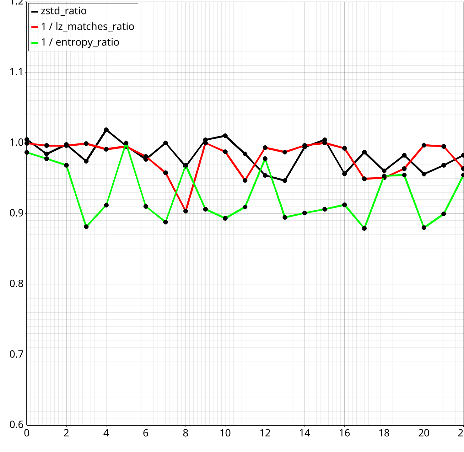
Use the extra split when the files are smaller!!
If you're optimizing for compression ratio only (e.g. file downloads), then always apply if smaller. Otherwise, only apply if the difference is significant enough as to not outweigh decompression speed.
Use the Est/Zstd Agreement on Better Group field
It tells you how often the 'estimate' function agrees with actual zstd results on whether the
split group is better than non-split. Above we get 72.8%, so it guesses it right 3/4 of the time, roughly.
Adding a Custom Comparison
For more advanced transformations, you can define custom comparisons!
By using the compare_groups feature.
Simple Example
The previous transformations can be defined as the following
analysis:
  compare_groups:
    - name: dxt1_transforms
      description: Compare different arrangements of DXT1 block data
      baseline: # Original block format: Each block is [color0, color1, indices]
        - type: struct
          fields:
            - type: field
              field: color0
            - type: field
              field: color1
            - type: field
              field: indices
      comparisons:
        colors_then_indices: # All colors first, then all indices
          - { type: array, field: colors } # Same as original blog post
          - { type: array, field: indices }
        color0_color1_indices: # All (split) colors first, then all indices
          - { type: array, field: color0 } # Introduced in this post.
          - { type: array, field: color1 }
          - { type: array, field: indices }
Which gives you the following output in the tool:
dxt1_transforms: Compare different arrangements of DXT1 block data
  Overall Est/Zstd Agreement on Best Group: 79.2%
  Base Group:
    Size: 20015319
    LZ, Entropy: (9429814, 6.78)
    Base (est/zstd): 13505214/13420865

  colors_then_indices Group:
    Size: 20015319
    LZ, Entropy: (11350940, 6.78)
    Comp (est/zstd): 11840362/11767256
    Ratio (zstd): 87.7%
    Diff (zstd): -1653608

  color0_color1_indices Group:
    Size: 20015319
    LZ, Entropy: (11571464, 6.78)
    Comp (est/zstd): 11743347/11698334
    Ratio (zstd): 87.2%
    Diff (zstd): -1722530
Example 1: Interleaving Colours with Mixed Representations
Convert from [R0 R1] [G0 G1] [B0 B1] to [R0 G0 B0] [R1 G1 B1] format.
compare_groups:
  colour_conversion:
      description: "Rearrange interleaved colour channels from [R0 R1] [G0 G1] [B0 B1] to [R0 G0 B0] [R1 G1 B1]."
      baseline: # Original colour format
        - { type: array, field: R } # reads all 'R' values from input
        - { type: array, field: G } # reads all 'G' values from input
        - { type: array, field: B } # reads all 'B' values from input
      comparisons:
        split_components: # R0 G0 B0. Repeats until no data written.
          - type: struct
            fields:
              - { type: field, field: R } # reads 1 'R' value from input
              - { type: field, field: G } # reads 1 'G' value from input
              - { type: field, field: B } # reads 1 'B' value from input
In this case, interleaved format is usually better with regards to compression.
Example 2: Converting 7-bit to 8-bit Colours with Padding
Convert a 7-bit color value to an 8-bit representation by adding a padding bit.
compare_groups:
  convert_7_to_8_bit:
    description: "Adjust 7-bit color channel to 8-bit by appending a padding bit."
    baseline: # Original 7-bit format (R, R, R)
      - { type: array, field: color7 } # reads all '7-bit' colours from input
    comparisons:
      padded_8bit: # 8-bit format with padding (R+0, R+0, R+0)
        - type: struct
          fields:
            - { type: field, field: color7 } # reads 1 '7-bit' colour from input
            - { type: padding, bits: 1, value: 0 } # appends padding bit
In this case, counterintuitively, extending to 8 bits often improves compression ratio; since compressors work on byte aligned data.
Example 3: Aligning Color Bits
Truncating 18-bit colours to 16-bit
Another case of byte aligning to improve compression ratio.
compare_groups:
  - name: convert_666_to_655
    description: "Convert colours from 666 to 655 format with lossy and lossless options"
    baseline: # 18-bit 666 colour
      - { type: array, field: color666 }
    comparisons:
      lossy_655: # 16-bit 655 colour (dropping '1' bit)
        - type: struct
          fields:
            - { type: field, field: color666, bits: 6 } # R (6-bit)
            - { type: field, field: color666, bits: 5 } # G (5-bit)
            - { type: skip, field: color666, bits: 1 }  # Discard remaining G bit
            - { type: field, field: color666, bits: 5 } # B (5-bit)
            - { type: skip, field: color666, bits: 1 }  # Discard remaining B bit
      lossless_655: # 16-bit 655 colour plus dropped bits stored separately
        - type: struct # Main 655 colour data
          fields:
            - { type: field, field: color666, bits: 6 } # R (6-bit)
            - { type: field, field: color666, bits: 5 } # G (5-bit)
            - { type: skip, field: color666, bits: 1 }  # Skip G low bit
            - { type: field, field: color666, bits: 5 } # B (5-bit)
            - { type: skip, field: color666, bits: 1 }  # Skip B low bit
        - { type: array, field: color666, offset: 11, bits: 1 } # All G low bits
        - { type: array, field: color666, offset: 17, bits: 1 } # All B low bits
This example shows two approaches to converting from 666 to 655 color format:
- A lossy conversion that drops two '1' bits.
- A lossless conversion that preserves the remaining bits in separate arrays after the array of 655 colour values.
Automatic Starting Offset & Length Detection
Up till now we've assumed that the input data consists of only what we're analyzing
This may not always be the case.
For example, you may want to skip a file header, or only handle a certain known part of a file.
In our case, for .DDS files, we can define a simple set of checks for BC1 format.
conditional_offsets:
  - offset: 0x80  # DXT1 data starts at 128 bytes
    conditions:
      - byte_offset: 0x00  # file magic
        bit_offset: 0
        bits: 32
        value: 0x44445320  # DDS magic

      - byte_offset: 0x54  # fourCC field position
        bit_offset: 0
        bits: 32
        value: 0x44585431  # 'DXT1' fourCC code
This will automatically set the starting offset of the data being analyzed to 0x80, if bytes or bits at specific locations match. The length should run till the end of the data.
There are offset and length parameters in the CLI
We've just conveniently left them out of the examples, and this is why.
Need a way to set fixed length? Submit a PR!
Chances are it'll be a while till I'll need it, so I haven't added it yet.
More Advanced Example
This checks multiple locations among the headers, and accepts either SRGB or regular format.
conditional_offsets:
  # BC7 format detection (UNORM)
  - offset: 0x94  # BC7 data starts at 148 bytes
    conditions:
      - byte_offset: 0x00 # file magic
        bit_offset: 0
        bits: 32
        value: 0x44445320 # DDS magic
      - byte_offset: 0x54 # ddspf.dourCC
        bit_offset: 0
        bits: 32
        value: 0x44583130 # DX10 header
      - byte_offset: 0x80 # ds_header_dxt10.dxgiFormat
        bit_offset: 0
        bits: 32
        value: 0x62000000 # DXGI_FORMAT_BC7_UNORM
  # BC7 format detection (UNORM_SRGB)
  - offset: 0x94  # BC7 data starts at 148 bytes
    conditions:
      - byte_offset: 0x00 # file magic
        bit_offset: 0
        bits: 32
        value: 0x44445320 # DDS magic
      - byte_offset: 0x54 # ddspf.dourCC
        bit_offset: 0
        bits: 32
        value: 0x44583130 # DX10 header
      - byte_offset: 0x80 # ds_header_dxt10.dxgiFormat
        bit_offset: 0
        bits: 32
        value: 0x63000000 # DXGI_FORMAT_BC7_UNORM_SRGB
Per File Statistics
When analyzing a directory, you may add the --output flag to output per-file statistics.
For example:
cargo run --release analyze-directory --output reports --schema schemas/dxt1-block.yaml "202x-architecture-10.01" -f concise
Will output per-file statistics in the reports directory.
These come in the form of CSV files and plots.
Plot Generation
Plots are generated for every split_comparison and custom_comparison.
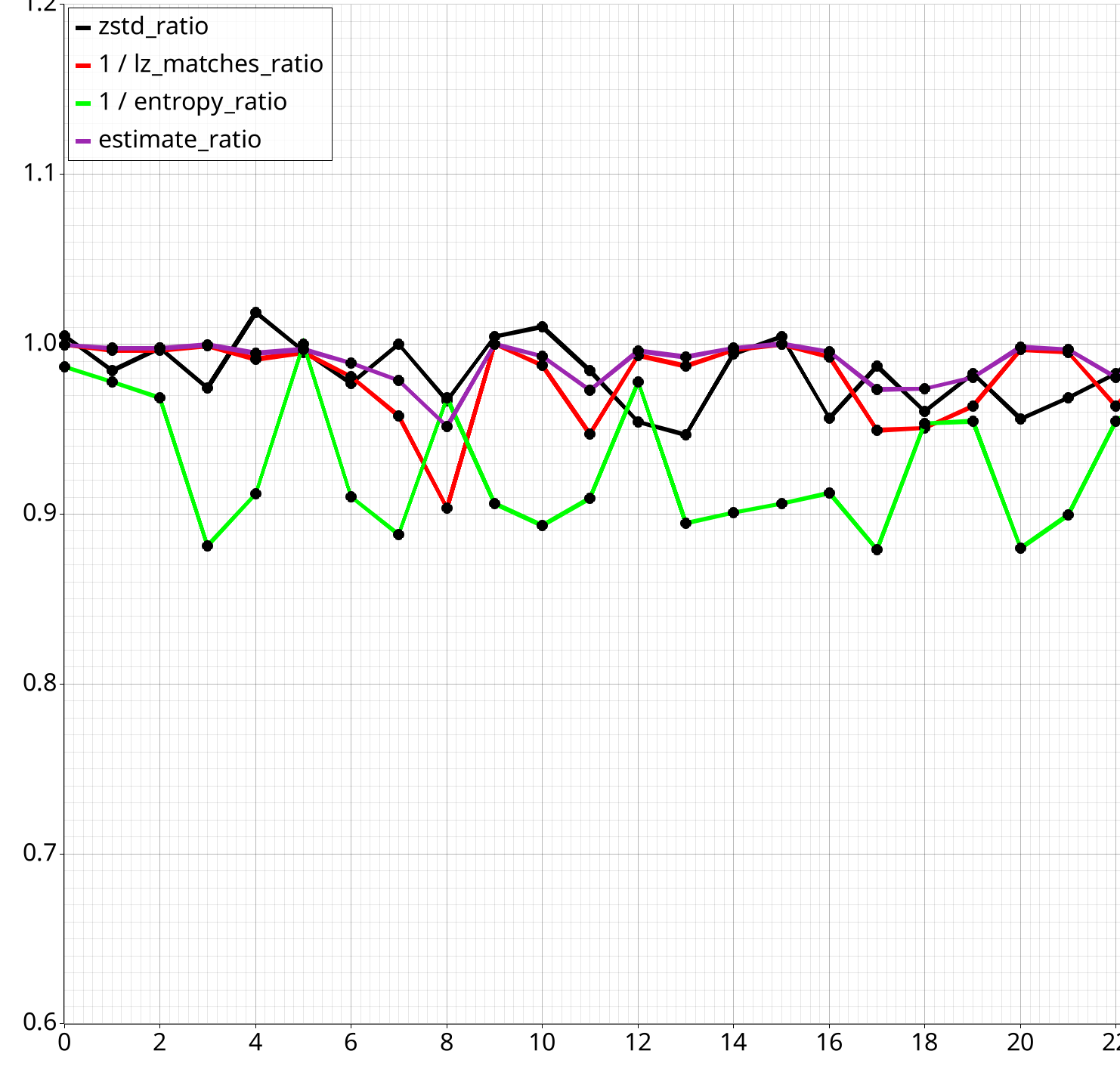
There may be multiple variants per comparison, e.g. like the one above with the 'estimate' function. This helps with readability, sometimes you want to exclude some info.
CSV Output
Per-file statistics are output in CSV format.
For example you can find...
Stats for Each Field
Same as in CLI output, but not aggregated.
| name | full_path | depth | entropy | lz_matches | lz_matches_pct | estimated_size | zstd_size | original_size | estimated_size_pct | zstd_size_pct | original_size_pct | zstd_ratio | lenbits | unique_values | bit_order | file_name |
|---|---|---|---|---|---|---|---|---|---|---|---|---|---|---|---|---|
| colors | colors | 0 | 4.874987 | 22330102 | 0.9679138 | 8528692 | 5871479 | 22369628 | 0.2827256 | 0.2073072 | 0.5 | 0.2624755 | 32 | 0 | Msb | winterholdwall02.dds |
| colors | colors | 0 | 4.876666 | 22254764 | 0.9761022 | 8548851 | 5504367 | 22369628 | 0.2832391 | 0.1943305 | 0.5 | 0.2460643 | 32 | 0 | Msb | winterholdfloor01.dds |
| colors | colors | 0 | 5.127527 | 22183499 | 0.9949356 | 9005741 | 6532419 | 22369628 | 0.2932818 | 0.2247291 | 0.5 | 0.2920218 | 32 | 0 | Msb | winterholdfloor02.dds |
Bit Statistics
This shows how often each bit in a field is set to zero or one
index0:
| bit_offset | zero_count | one_count | ratio |
|---|---|---|---|
| 0 | 140489327 | 172250038 | 0.4492218 |
| 1 | 167653801 | 145085564 | 0.5360815 |
Value Statistics
This shows the probability of each value occurring in a given field
index0:
| value | count | ratio |
|---|---|---|
| 3 | 86242725 | 0.2757655 |
| 2 | 86007313 | 0.2750128 |
| 0 | 81646488 | 0.2610688 |
| 1 | 58842839 | 0.1881530 |
Split/Custom Comparisons
Same as in CLI output, but with a bit more info and not aggregated.
| name | file_name | size | base lz | comp lz | base est | base zstd | comp est | comp zstd | ratio est | ratio zstd | diff est | diff zstd | base group lz | comp group lz | base group entropy | comp group entropy | max comp lz diff | max comp entropy diff |
|---|---|---|---|---|---|---|---|---|---|---|---|---|---|---|---|---|---|---|
| split_colors | winterholdwall02.dds | 22369628 | 22330102 | 22337863 | 8528692 | 5871479 | 8526919 | 5900243 | 0.9997921 | 1.0048989 | -1773 | 28764 | 22330102 | 11173030|11162725 | 4.87 | 4.64|4.70 | 1.00 | 0.06 |
| split_colors | winterholdfloor01.dds | 22369628 | 22254764 | 22328220 | 8548851 | 5504367 | 8532059 | 5417979 | 0.9980358 | 0.9843056 | -16792 | -86388 | 22254764 | 11157143|11166978 | 4.88 | 4.69|4.58 | 1.00 | 0.10 |
| split_colors | winterholdfloor02.dds | 22369628 | 22183499 | 22263057 | 9005741 | 6532419 | 8986619 | 6517815 | 0.9978767 | 0.9977644 | -19122 | -14604 | 22183499 | 11118891|11136522 | 5.13 | 4.77|4.92 | 1.00 | 0.16 |
| split_colors | winterholdrubble01.dds | 22369628 | 22317563 | 22339474 | 8018446 | 6212103 | 8013740 | 6051193 | 0.9994131 | 0.9740973 | -4706 | -160910 | 22317563 | 11157699|11178604 | 4.58 | 4.30|3.79 | 1.00 | 0.51 |
| split_colors | riftenlogsiding01.dds | 22369628 | 21827972 | 22025297 | 9701135 | 7449007 | 9650526 | 7587915 | 0.9947832 | 1.0186479 | -50609 | 138908 | 21827972 | 10955631|11055353 | 5.47 | 5.66|5.17 | 1.01 | 0.50 |
Filtering of Input Data
Sometimes you want to only analyze structures that fit a certain criteria.
For example, when dealing with BC7 Texture, each 'block' starts off with a number of bits that defines its mode.
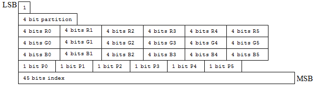 Mode 1:
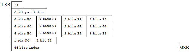 Mode 2:
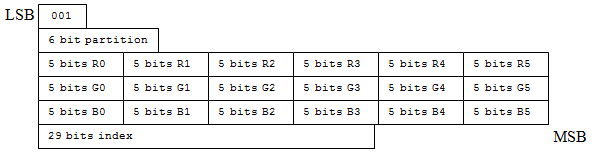
Image from MSDN BC7 Format Mode Reference.
root:
  type: group
  # Filter out to only Mode0 blocks, with start with a single '1' bit.
  # https://learn.microsoft.com/en-us/windows/win32/direct3d11/bc7-format-mode-reference#mode-0
  skip_if_not:
  - byte_offset: 0
    bit_offset: 0
    bits: 1
    value: 1

  # Note: We filter out at root, so `mode0_block` reports the correct size of only Mode0 blocks
  #       in the file.
  fields:
    mode0_block:
      # rest of block...
Size Predictor / Estimator
Certain parts of the output refer to an 'estimate'
You would have seen this in Split Comparisons, Custom Comparisons, and Plots.
This estimate is based on the quickly estimate the file size segment of the previous blog post. Using the following function.
pub fn size_estimate(params: SizeEstimationParameters) -> usize {
    // Calculate expected bytes after LZ
    let bytes_after_lz = params.data_len
        - (params.num_lz_matches as f64 * params.lz_match_multiplier) as usize;

    // Calculate expected bits and convert to bytes
    (bytes_after_lz as f64 * params.entropy * params.entropy_multiplier).ceil()
        as usize / 8
}
It takes file size, subtracts a multiple of lz_matches, and then estimates gains from entropy
coding step; by applying a multiplier to the file's entropy.
Stats such as lz_matches are provided by lossless-transform-utils (from last blog post).
Use an estimate like this to determine if to apply a lossless transform
Is the estimated size smaller? If so, apply the transform.
Size estimator function can be replaced via API
Brute Forcing The Parameters
Pass --brute-force-lz-params to directory analysis (in CLI) to auto find optimal parameters
This will give you a printout like:
=== Split Comparison Parameter Optimization Results ===
| Comparison Name | Group | LZ Multiplier | Entropy Multiplier |
| --------------- | ----- | ------------- | ------------------ |
| split_colors    | G1    | 0.5809        | 1.1670             |
|                 | G2    | 0.5727        | 1.1650             |

=== Custom Comparison Parameter Optimization Results ===
| Comparison Name | Group | LZ Multiplier | Entropy Multiplier |
| --------------- | ----- | ------------- | ------------------ |
| dxt1_transforms | BASE  | 0.533         | 1.000              |
|                 | 0     | 0.598         | 1.045              |
|                 | 1     | 0.586         | 1.038              |
Which shows you the best parameters for each split and group comparison. These are brute forced on all threads.
When the brute force option is set in the CLI, the results of analysis will automatically use the computed results.
split_colors: 'Compare regular interleaved colour format `colors` against their split components `color0` and `color1`'
  Base (est/zstd): 3634154/3567275 # 👈 updated
  Comp (est/zstd): 3503905/3498364 # 👈 updated
  Est/Zstd Agreement on Better Group: 72.8% # 👈 updated

dxt1_transforms: 'Compare different arrangements of DXT1 block data'
  Overall Est/Zstd Agreement on Best Group: 79.2% # 👈 updated
  Base Group:
    Base (est/zstd): 13505214/13420865 # 👈 updated

  colors_then_indices Group:
    Comp (est/zstd): 11840362/11767256 # 👈 updated

  color0_color1_indices Group:
    Comp (est/zstd): 11743347/11698334 # 👈 updated
The brute force is optimized to maximize the Est/Zstd Agreement on Better Group statistic
We compromise on size accuracy (a miniscule amount) to get a better overall prediction of when a transform will be beneficial by applying a 'penalty'.
// If the ratios are on the opposite side of 1.0
// (i.e.) estimate thinks its worse, when its better, impose a 'killing'
// penalty by giving it max error.
let zstd_is_bigger = zstd_size > original_size;
let estimate_is_bigger = estimated_size as u64 > original_size;
if zstd_is_bigger != estimate_is_bigger {
    return f32::MAX as f64;
}
This is not adjustable as it's on a hot path; analysis time would increase significantly if made replaceable.
Estimator Accuracy (High Compression Level)
Small sample size, 125 files
Below is a reference set of results for split_colors.
On "202x-architecture-10.01", as per previous examples.
We compress the input with zstd level 19, then check the result of Est/Zstd Agreement on Better Group,
marking that result as Accuracy.
In this example, Accuracy result marks how often the estimate function agrees with zstd level 19
on whether ratio will improve as a result of splitting the colour channels.
| Method | Speed (MB/s) | Accuracy |
|---|---|---|
| Estimator | 1610-1700 | 74.4% |
| ZStd (lv 1) | 600-1250 | 79.2% |
| ZStd (lv 2) | 340-530 | 81.6% |
| ZStd (lv 3) | 183 | 84.0% |
| ZStd (lv 4) | 154 | 84.8% |
| ZStd (lv 5) | 100 | 86.4% |
| ZStd (lv 6) | 81 | 88.0% |
| ZStd (lv 7) | 75 | 90.4% |
| ZStd (lv 8) | 69 | 91.2% |
| ZStd (lv 9) | 64 | 90.4% |
| ZStd (lv 10) | 48 | 93.6% |
The Speed column is a single threaded estimate, I don't have an exact benchmark for this; it will
vary very, very slightly between files.
In general, as a general rule of thumb, the accuracy of the estimator is generally comparable to that of
using ZStd level 1; but at double the speed. Use it for 'real-time' compression/decompression scenarios
(see below).
You can replace estimator in CompressionOptions struct.
This is how we measured for zstd here.
When compressing at high levels, use low levels of same algorithm as the estimator.
Although fast, the 'estimate' lacks accuracy for high compression levels.
Keep the estimate for low compression levels.
Using low compression levels you can still achieve <10% overhead, while having much more accurate results.
Correct Positives & False Positives (High Compression Level)
Another useful statistics are false positives and correct positives
A 'correct positive' is when we predicted group2 / comp group is better, and it indeed was.
A 'false positive' is when we predicted it was better, but it was not.
Another, perhaps better statistic is 'false positives'
This is the amount of times the estimator thought the ratio would improve (with group2 / comp group)
, but it did not actually improve.
| Method | Speed (MB/s) | False Positives | Correct Positives |
|---|---|---|---|
| Estimator | 1610-1700 | 24.8% | 72.8% |
| ZStd (lv 1) | 600-1250 | 20.0% | 72.8% |
| ZStd (lv 7) | 75 | 9.6% | 73.6% |
The idea here is 'you may disagree if ratio improves', but being wrong, saying the ratio will improve, when it in fact won't is more dangerous than being wrong.
Estimator Accuracy (Mid Compression Level)
Below is a reference set of results for split_colors.
On my entire BC1 data set. Not just the mod above.
For low compression levels, the 'estimate' function is competitive with level 1.
This time we're compression with ZStd level 9, and measuring the results.
| Method | Speed (MB/s) | Accuracy |
|---|---|---|
| Estimator | 1610-1700 | 80.0% |
| ZStd (lv 1) | 600-1250 | 83.8% |
| ZStd (lv 2) | 340-530 | 85.9% |
| ZStd (lv 3) | 183 | 89.9% |
Level 3 provided for completeness; it has too much overhead in practice.
Correct Positives & False Positives (Mid Compression Level)
The estimate function tends to produce less false positives.
Which evens out the less correct positives.
| Method | Speed (MB/s) | False Positives | Correct Positives |
|---|---|---|---|
| Estimator | 1610-1700 | 10.0% | 60.2% |
| ZStd (lv 1) | 600-1250 | 13.5% | 67.5% |
| ZStd (lv 2) | 340-530 | 13.0% | 69.0% |
| ZStd (lv 3) | 183 | 9.2% | 69.2% |
Estimator Accuracy vs BZip3
What if we estimate against something that isn't LZ based?
Comparing effectiveness on BZip3 instead of ZStandard
This requires a simple code edit, to change get_zstd_compressed_size to
a different compression algorithm.
May expose this via function pointer in future.
| Method | Speed (MB/s) | Accuracy |
|---|---|---|
| Estimator | 1610-1700 | 84.8% |
| ZStd (lv 1) | 600-1250 | 10.4% |
| ZStd (lv 3) | 183 | 15.2% |
| BZip3 | 12 | 100.0% |
| Method | Speed (MB/s) | False Positives | Correct Positives |
|---|---|---|---|
| Estimator | 1610-1700 | 12.8% | 2.4% |
| ZStd (lv 1) | 600-1250 | 88.8% | 4.0% |
| ZStd (lv 3) | 183 | 84.8% | 4.8% |
| BZip3 | 12 | 0% | 100% |
Using LZ Based solutions, including ZStandard on non-LZ Based bzip3 does not yield good results.
Because the Burrows Wheeler Transform is fundamentally different than an LZ based algorithm.
Always tread with caution. Splitting here often hurts bz3.
Results on entire data set (1943 files):
| Method | Speed (MB/s) | Accuracy |
|---|---|---|
| Estimator | 1610-1700 | 84.9% |
| Method | Speed (MB/s) | False Positives | Correct Positives |
|---|---|---|---|
| Estimator | 1610-1700 | 5.0% | 5.6% |
Alternate Method (Mid Compression Level)
We can also compare sizes of just the separate color0, color1 fields being split.
| Method | Speed (MB/s) | Accuracy |
|---|---|---|
| Estimator | 1610-1700 | 94.4% |
| ZStd (lv 1) | 600-1250 | 98.0% |
| Method | Speed (MB/s) | False Positives |
|---|---|---|
| Estimator | 1610-1700 | 2.3% |
| ZStd (lv 1) | 600-1250 | 0.6% |
You can subtract the sizes of the 2 split segments, and decide to split if they differ significantly enough as a rule of thumb. But I would not suggest, rather look at raw LZ and entropy numbers here.
API Usage
A Rust crate is provided, though bear in mind this is primarily a CLI tool.
# Cargo.toml
[dependencies]
struct-compression-analyzer = "0.1.0"
Example usage:
use struct_compression_analyzer::results::PrintFormat;
use struct_compression_analyzer::schema::Schema;
use struct_compression_analyzer::analyzer::SchemaAnalyzer;
use struct_compression_analyzer::analyzer::CompressionOptions;
use std::path::Path;

fn main() -> anyhow::Result<()> {
    // Load the schema
    let schema = Schema::load_from_file(Path::new("schema.yaml"))?;

    // Set the options
    let options = CompressionOptions::default();

    // Create an analyzer
    let mut analyzer = SchemaAnalyzer::new(&schema, options);

    // Add data to analyze
    analyzer.add_entry(&[0x01, 0x02, 0x03])?;

    // Generate results
    let results = analyzer.generate_results()?;

    // Print the results
    results.print(&schema, PrintFormat::Concise, false);

    Ok(())
}
For more detailed API documentation, see the rust docs.
Each module has its own documentation, so use the sidebar 😉.
No API stability is guaranteed whatsoever, this is a one-off few weekend project; and is primarily a CLI tool.
Missing Features?
A few, possibly.
Will add them as needed in future endeavours.
If you need them, please PR them!! Don't wait!!
- Custom lengths for conditional offsets
- Ability to handle variable sized structs.
- e.g. Length prefixed arrays within structs.
The sources and documentation for this project can be found at: - GitHub Repository - Documentation